Insertion Sort

Insertion sort:


Insertion sort is a simple sorting algorithm, a comparison sort in which the sorted array (or list) is built one entry at a time. It is much less efficient on large lists than more advanced algorithms such as quicksort, heapsort, or merge sort. However, insertion sort provides several advantages:

• Simple implementation
• Efficient for (quite) small data sets
• Adaptive, i.e. efficient for data sets that are already substantially sorted: the time complexity is O(n + d), where d is the number of inversions
• More efficient in practice than most other simple quadratic, i.e. O(n²) algorithms such as selection sort or bubble sort; the best case (nearly sorted input) is O(n)
• Stable, i.e. does not change the relative order of elements with equal keys
• In-place, i.e. only requires a constant amount O(1) of additional memory space
• Online, i.e. can sort a list as it receives it.

Most humans when sorting—ordering a deck of cards, for example—use a method that is similar to insertion sort.

Algorithm

Every repetition of insertion sort removes an element from the input data, inserting it into the correct position in the already-sorted list, until no input elements remain. The choice of which element to remove from the input is arbitrary, and can be made using almost any choice algorithm.
Sorting is typically done in-place. The resulting array after k iterations has the property where the first k + 1 entries are sorted. In each iteration the first remaining entry of the input is removed, inserted into the result at the correct position, thus extending the result:


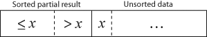
becomes


with each element greater than x copied to the right as it is compared against x.
The most common variant of insertion sort, which operates on arrays, can be described as follows:

1. Suppose there exists a function called Insert designed to insert a value into a sorted sequence at the beginning of an array. It operates by beginning at the end of the sequence and shifting each element one place to the right until a suitable position is found for the new element. The function has the side effect of overwriting the value stored immediately after the sorted sequence in the array.
2. To perform an insertion sort, begin at the left-most element of the array and invoke Insert to insert each element encountered into its correct position. The ordered sequence into which the element is inserted is stored at the beginning of the array in the set of indices already examined. Each insertion overwrites a single value: the value being inserted.

Pseudocode of the complete algorithm follows, where the arrays are zero-based and the for-loop includes both the top and bottom limits (as in Pascal):

insertionSort(array A)
begin
    for i := 1 to length[A]-1 do
    begin
        value := A[i];
        j := i - 1;
        done := false;
        repeat
            if A[j] > value then
            begin
                A[j + 1] := A[j];
                j := j - 1;
                if j < 0 then
                    done := true;
            end
            else
                done := true;
        until done;
        A[j + 1] := value;
    end;
end;

Below is the pseudocode for insertion sort (as in C):

1. for j ← to length(A)
2. do key ← A[ j ]
3. > A[ j ] is added in the sorted sequence A[1, .. j-1]
4. i ← j - 1
5. while i >= 0 and A [ i ] > key
6. do A[ i +1 ] ← A[ i ]
7. i ← i -1
8. A [i +1] ← key

 Best, worst, and average cases

Graphical example.

The best case input is an array that is already sorted. In this case insertion sort has a linear running time (i.e., Θ(n)). During each iteration, the first remaining element of the input is only compared with the right-most element of the sorted subsection of the array.
The worst case input is an array sorted in reverse order. In this case every iteration of the inner loop will scan and shift the entire sorted subsection of the array before inserting the next element. For this case insertion sort has a quadratic running time (i.e., O(n²)).
The average case is also quadratic, which makes insertion sort impractical for sorting large arrays. However, insertion sort is one of the fastest algorithms for sorting very small arrays, even faster than quick sort; indeed, good quick sort implementation use insertion sort for arrays smaller than a certain threshold, also when arising as subproblems; the exact threshold must be determined experimentally and depends on the machine, but is commonly around ten.
Example: The following table shows the steps for sorting the sequence {5, 7, 0, 3, 4, 2, 6, 1}. For each iteration, the number of positions the inserted element has moved is shown in parentheses. Altogether this amounts to 17 steps.

5 7 0 3 4 2 6 1 (0)

5 7 0 3 4 2 6 1 (0)
0 5 7 3 4 2 6 1 (2)
0 3 5 7 4 2 6 1 (2)
0 3 4 5 7 2 6 1 (2)
0 2 3 4 5 7 6 1 (4)
0 2 3 4 5 6 7 1 (1)
0 1 2 3 4 5 6 7 (6)

Comparisons to other sorting algorithms

Insertion sort is very similar to selection sort. As in selection sort, after k passes through the array, the first k elements are in sorted order. For selection sort these are the k smallest elements, while in insertion sort they are whatever the first k elements were in the unsorted array. Insertion sort's advantage is that it only scans as many elements as needed to determine the correct location of the k+1^th element, while selection sort must scan all remaining elements to find the absolute smallest element.
Calculations show that insertion sort will usually perform about half as many comparisons as selection sort. Assuming the k+1^th element's rank is random, insertion sort will on average require shifting half of the previous k elements, while selection sort always requires scanning all unplaced elements. If the input array is reverse-sorted, insertion sort performs as many comparisons as selection sort. If the input array is already sorted, insertion sort performs as few as n-1 comparisons, thus making insertion sort more efficient when given sorted or "nearly-sorted" arrays.
While insertion sort typically makes fewer comparisons than selection sort, it requires more writes because the inner loop can require shifting large sections of the sorted portion of the array. In general, insertion sort will write to the array O(n²) times, whereas selection sort will write only O(n) times. For this reason selection sort may be preferable in cases where writing to memory is significantly more expensive than reading, such as with EEPROM or flash memory.
Some divide-and-conquer algorithms such as quicksort and mergesort sort by recursively dividing the list into smaller sublists which are then sorted. A useful optimization in practice for these algorithms is to use insertion sort for sorting small sublists, where insertion sort outperforms these more complex algorithms. The size of list for which insertion sort has the advantage varies by environment and implementation, but is typically between eight and twenty elements.

 Variants

D.L. Shell made substantial improvements to the algorithm; the modified version is called Shell sort. The sorting algorithm compares elements separated by a distance that decreases on each pass. Shell sort has distinctly improved running times in practical work, with two simple variants requiring O(n^3/2) and O(n^4/3) running time.
If the cost of comparisons exceeds the cost of swaps, as is the case for example with string keys stored by reference or with human interaction (such as choosing one of a pair displayed side-by-side), then using binary insertion sort may yield better performance. Binary insertion sort employs a binary search to determine the correct location to insert new elements, and therefore performs comparisons in the worst case, which is Θ(n log n). The algorithm as a whole still has a running time of Θ(n²) on average because of the series of swaps required for each insertion.
The number of swaps can be reduced by calculating the position of multiple elements before moving them. For example, if the target position of two elements is calculated before they are moved into the right position, the number of swaps can be reduced by about 25% for random data. In the extreme case, this variant works similar to merge sort.
To avoid having to make a series of swaps for each insertion, the input could be stored in a linked list, which allows elements to be inserted and deleted in constant-time. However, performing a binary search on a linked list is impossible because a linked list does not support random access to its elements; therefore, the running time required for searching is O(n²). If a more sophisticated data structure (e.g., heap or binary tree) is used, the time required for searching and insertion can be reduced significantly; this is the essence of heap sort and binary tree sort.
In 2004 Bender, Farach-Colton, and Mosteiro published a new variant of insertion sort called library sort or gapped insertion sort that leaves a small number of unused spaces (i.e., "gaps") spread throughout the array. The benefit is that insertions need only shift elements over until a gap is reached. The authors show that this sorting algorithm runs with high probability in O(n log n) time.^[2]